Case Study 2 · Whole-scalp spectral analysis of resting-state EEG

An exploratory, whole-scalp look at resting-state EEG spectra and global cognition — no a priori restriction to a single frequency band or region, analysed with cluster-based permutation testing.

See the code

204 channels × 159 freqs Cluster permutation Real EEG spectra

Research question

Does the spectral profile of resting-state EEG relate to global cognitive functioning, without restricting the analysis in advance to a specific frequency band or region?

Where Case Study 1 reduces the EEG signal to four theory-driven scalar features, this case study keeps the full power spectral density (PSD, 1–40 Hz, every channel) and asks broadly where — across the whole scalp and spectrum — resting EEG power relates to global cognition (MoCA). It is motivated by a well-established clinical observation: right-hemisphere stroke is frequently accompanied by pathological EEG slowing (more delta/theta power over the affected region) that tracks the severity of impairment (Finnigan & Van Putten, 2013).

Data — and an important disclosure

• The EEG spectra are real, anonymised recordings from the PATHS study (Welch's method, 1–40 Hz), authorised for publication here.
• The neuropsychological table (age, sex, CRIq, MoCA) is synthetic, as in Case Study 1.
• Because the two do not come from the same assessment, the moca column was deliberately linked to a real, montage-based property of each EEG recording (see data/generate_datasets.ipynb for the full, explicit disclosure). The resulting brain–behaviour association should not be read as a real clinical finding — it exists so this case study has a real spectrum to analyse and something genuine to recover.

Pipeline

1. Data Wrangling

• Strictly align PSD array with neuropsychological table
• Spectrum data-quality checks
• Log-power distribution check

2. Analysis

• Baseline model (Case-Study-1-style, for contrast)
• Mass-univariate partial correlation
• Cluster-based permutation (primary + secondary)
• Exploratory per-band breakdown

3. Export

• Figures (PNG)
• Tables (CSV + Excel)

A taste of the results

• 

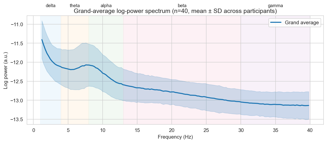
  The real grand-average EEG spectrum: a 1/f-like decay with a visible alpha bump — a first sanity check that the recordings look like EEG.

• 

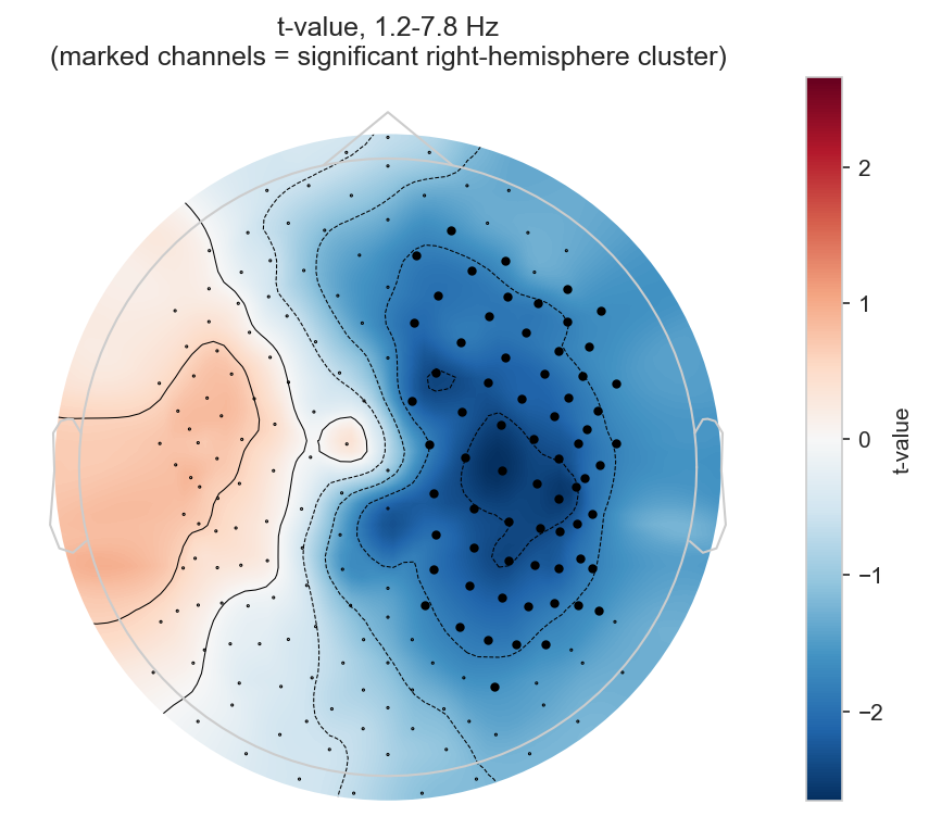
  Where the significant effect is: a right-lateralised, low-frequency cluster (marked channels), shown against real data on both hemispheres.

Key takeaway

The primary, whole-spectrum test does not survive correction at n=40 — an honest illustration of the paper's own caveat that cluster-based permutation is relatively underpowered at this sample size. A secondary, pre-registered test restricted to the hypothesised region (right hemisphere, delta/theta) does recover a significant cluster. Reporting both, rather than only the one that "worked", is what keeps the secondary result meaningful — the same a-priori-vs-post-hoc logic Case Study 1 teaches for choosing predictors, applied here to choosing where to look. An exploratory breakdown by individual frequency band (Section 2.7 of the code) makes the trade-off concrete: none of the five canonical bands survives correction on its own, which is exactly why the secondary test pools delta and theta together.

See the code

Exported results, ready to open in Excel or re-use elsewhere:

• All tables — one workbook, one sheet each
• Descriptive statistics (CSV)
• Cluster results — primary & secondary (CSV)
• Baseline model (CSV)
• Per-band breakdown, exploratory (CSV)

The code and raw data also live in the [REDACTED] repository, under python/CaseStudy_2/, r/case2/, and data/.

Strengths and limitations

Strengths — no a priori commitment to a specific band or region, able to recover a distributed, low-frequency, right-hemisphere pattern that no single ERP feature (Case Study 1) would capture; respects the real spatial and spectral dependency structure of the signal.

Limitations — computationally heavier than the GLM-based approach of Case Study 1; statistically demanding, since cluster-based permutation is relatively underpowered at a sample size like this one, so only fairly marked associations are likely to survive; a significant secondary result is only meaningful because the restricted region was pre-registered before looking at the data — restricting only after seeing what "worked" would be the same circular reasoning Case Study 1 warns against, just at the level of search space instead of predictor selection.